
"Predicting Noise" A Minimal Simulation of Linear Regression on Asset Returns
A controlled experiment with normally distributed returns
Big stories, small signals
Markets move on stories geopolitical shifts, industrial policy, energy transitions, or supply-chain rewiring. Essays and newsletters that unpack these forces are compelling because they provide a narrative lens: they tell us why prices moved yesterday, or why an asset might outperform next quarter. They frame uncertainty in digestible terms and give the impression of understanding the forces at work.
But stories do not trade themselves. The market responds to numbers orders, flows, positions and even the most persuasive narrative cannot reliably convert insight into returns without a disciplined way to quantify it. The tension between story and signal is subtle: narratives are seductive and explanatory, but quantifiable signals are testable. One can feel certain about a trend in hindsight, yet that certainty often collapses under forward evaluation.
Before letting narratives seduce our models, it’s useful to ask a simpler, sharper question: what does our most basic predictive tool linear regression do in a world that offers almost nothing to predict?
This is not a dismissal of stories. Rather, it is an acknowledgment that the illusion of predictability is pervasive. Markets appear patterned in retrospect because humans seek coherence. Signals appear stronger than they are because narrative shapes attention. By first examining a controlled, minimal environment, we learn a valuable lesson: a trading signal can look competent even when the underlying predictability is weak or impossible.
Building the experiment
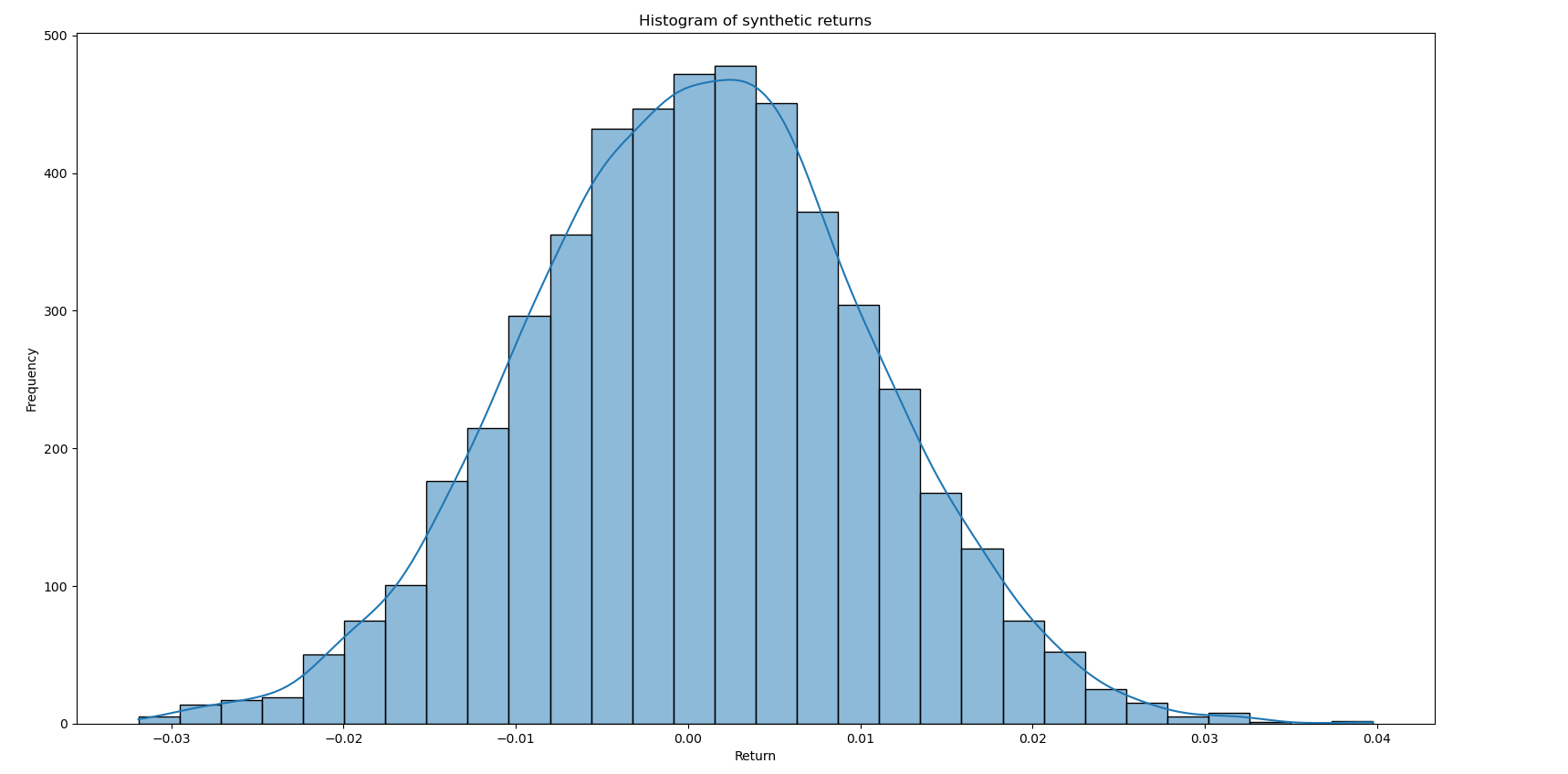
In this experiment, returns are drawn independently from a normal distribution, with a small mean and realistic volatility. The dataset is mostly randomness combined with a deliberately weak signal.
Linear regression is estimated using ordinary least squares (OLS) on the training subset, with no feature engineering, regularization, or optimization. Performance is then evaluated on the held-out test set.
Running the experiment
The training data set is a random distribution representing historical returns with parameters
mu = 0.0005
sigma = 0.01
with 500 samples values. The target signal is another random distribution with a similar structure but a slight positive bias to represent future values. The regression model is then trained using a sequential train test split, with a test hold out of 30%.
When examining the predicted values on the out of sample test, one can see that the model has much limited variation in its predictions. Why might this be the case?
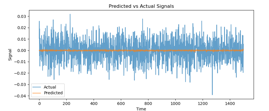
Evaluating the model: metrics and meaning
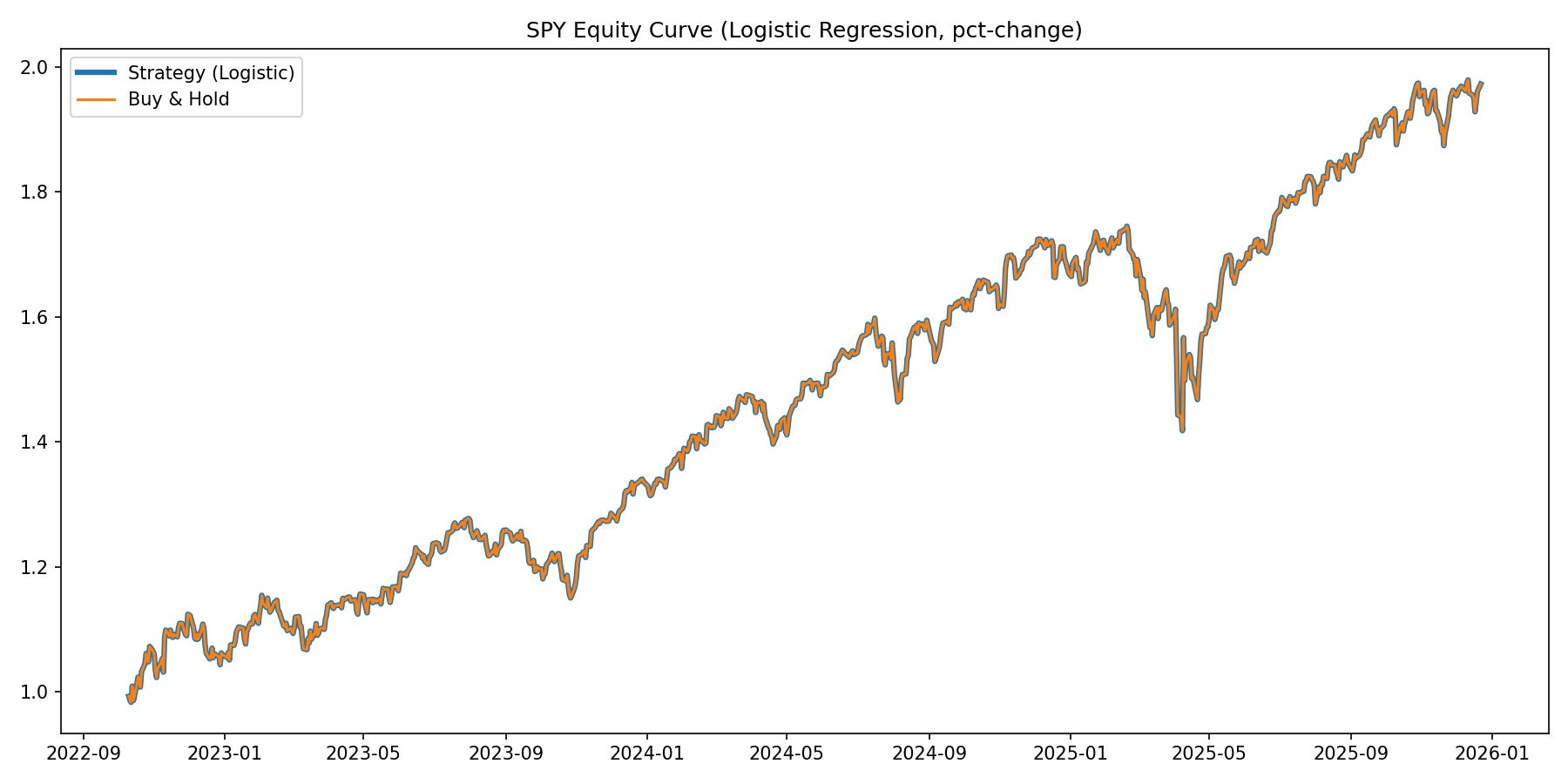
Because the data is drawn from a normal distribution, the model is essentially estimating the conditional mean of future returns. There is no real structure or predictable pattern beyond the small signal injected. By creating a small back test using the predicted return as a signal, we get a equity curve like this:

The model will only predict one signal (in this case go long) and present a culminative return that appears substantial given the distribution of the data (at least given the lower risk of this curve, the returns in this experiment not modeled to be exponentially weighted). In this case a return is generated because nothing about the assumptions changes and there is positive expectancy in the target dataset.
Relationship to the markets
A similar effect can be seen if a similar test is run using logistic regression (a linear classifier) to predict whether or not the next close in SPY will be positive. The model will only predict an up signal because on average the SPY goes up.
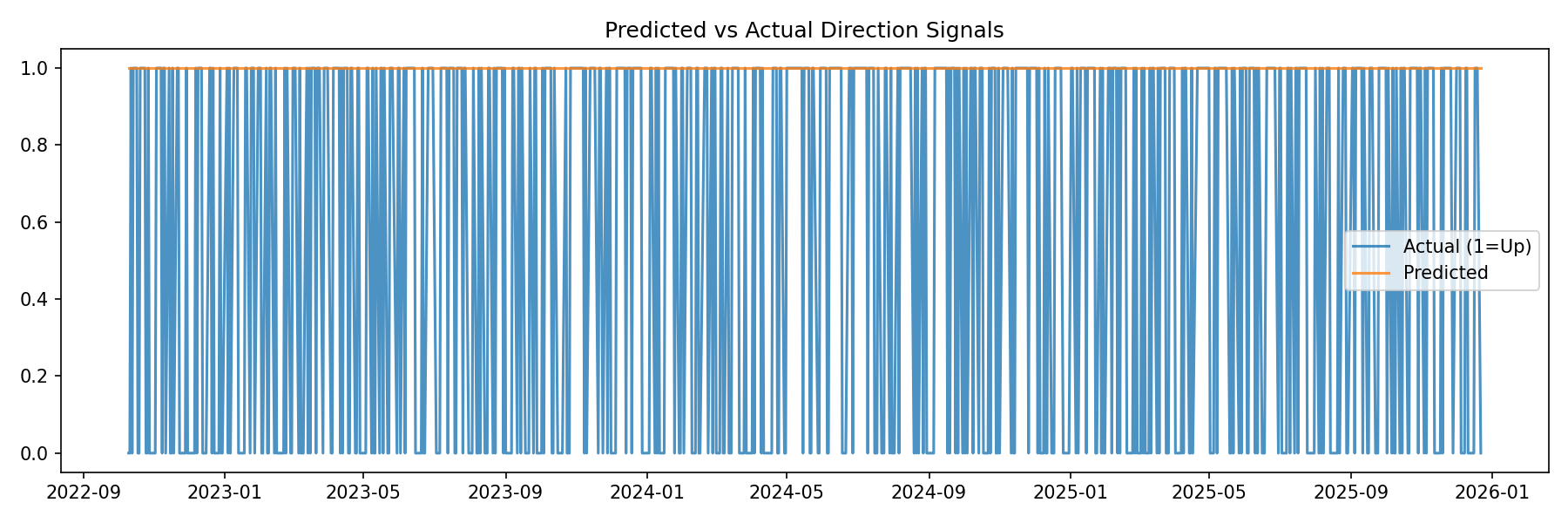
(As you can see the performance of this signal will be the same as buy and hold)
In this case because historically (and so far this year) the expectation of the SPY has remained positive, one could adjust a strategy based on a signal that on average the SPY goes up. Much like with certain dice games you can just keep playing to make money if the expectancy is positive. However these assumptions that the distributions of returns will not change (which isn’t true for markets).
Lessons
When the features are not really predictive, and based on historical values linear models (and many more really) will just learn the class weights that are most likely to occur, as seen in this small experiment. However, if we know that this is going to be stable (or we can find a way to predict that, which we will go over in future articles) a strategy can be optimized assuming these positive distributions remain.
Most models when trained with noise this high you can only really expect an R^2 of close to 0, meaning it is highly unlikely they will beat a naive predictor that returns the mean value of the target each time.
In future articles we will explore ways to reduce noise to have more predictive power in our features, different targets to select other than future returns that can generate a positive R^2 and many more methods to attack the world of stocks from a machine learning perspective.